How Vectors Are Produced In An Embedding Model
My first time hearing word ‘embedding’ was when I read a book about MLOps. MLOps is somewhat like DevOps but with additional tasks on Machine Learning workflows (deploying model, setting up feature pipeline, etc.). When I got into the “Feature Pipeline”, it introduced RAG (Retrieval Augmented Generation) which relies on an embedding model. The book explained what an embedding is and why it matters, which was helpful. However, when I saw a live demo of an embedding model in action, I got confused instead. Take this example,
sun -> [5.625; -2.911; 0.237]
“How come that is the result? What just happened? What those numbers represent?”
Seeing those numbers magically appear got me wondering what exactly was happening under the hood. Do these numbers have meaning or are they random? If they are random then how do they help the model, and how does the model know they aren’t random?
To find out, I spent time to learn how embedding works from the ground up.
Summary
The embedding I explore here is a word-level embedding, not a sentence-level embedding. It does not cover how transformers work. Instead, it uses a simplified training process to demonstrate how initially random vectors can be updated to encode useful relationships. The process does not reproduce any production-grade embedding model.
The number output by an embedding model is called Vector. An embedding vector is simply a set of spatial coordinates that places a concept inside a multi-dimensional room. Imagine setting up a kindergarten classroom. You have a list of kids along with their profiles—their personalities, interests, and past drama. To keep the room peaceful, you place kids who get along close together, facing the same direction, while keeping kids who clash far apart. Because these coordinates are normalized to a standard scale (keeping each kid’s distance fixed from the center of the room), their location values appear as floating-point decimals between -1.0 and 1.0.
Suppose we start with two kids placed at initial room coordinates like [0.5; -0.6; -0.8] and [0.7; 0.1; -0.2]. Because the model hasn’t learned who gets along yet, these starting positions are essentially random. As training progresses, the model learns their profile similarities and shifts their locations to [0.53; 0.10; -0.48] and [0.45; 0.20; -0.39].
What actually happened? The model moved the two kids closer together in the room and turned them to face the same way. In vector math, we measure this spatial alignment (their profile similarities) using two key metrics:
- Cosine similarity, which tracks how closely their directions match (getting closer to 1.0 as they align).
- Dot product, which combines both their directional alignment and distance to give an overall score of how strongly they belong in the same neighborhood.
To human eyes, raw coordinate numbers like [0.53; 0.10; -0.48] and [0.45; 0.20; -0.39] look unrelated. But through cosine similarity, the math proves they are facing the same direction. This doesn’t mean the model “understands” what these two words mean in a human sense. It simply means the model noticed how often they appeared together in the dataset—just like a teacher noticing two kids playing together every day on the playground, and deciding to assign them desks side by side. Should they sit together on the center? right corner? left corner? It doesn’t matter as long as they face the same direction.
Note: I’m not an AI researcher, scientist or an expert in this field. This blog is pure exploration and notes on what is my current understanding about components of AI. Please do clarify with someone who knows better.
Breaking Down the Magic Numbers
Recall the earlier example,
sun -> [5.625; -2.911; 0.237]
I still couldn’t understand what those numbers represented. I kept coming back to these questions:
- How are those numbers produced?
- What do they mean to the model?
- If those numbers are just random, why don’t we just assign a random number for each word instead of using an embedding model?
Thus, to answer the questions, I decided to write a minimal embedding model from scratch.
Talking About Data
What I didn’t realize about embedding models was, it requires training. Just like when I wrote a tokenizer before, the program needs to learn a pattern to create a model. Training requires a dataset, so we need a set of valid and meaningful sentences to be able to create an embedding model. During training, the model learns which words appear together in a sentence in the dataset. Those patterns are what we call “context”. Therefore, to build a proof of concept I use the following minimal dataset:
sun rise glow
moon sky star
star glow sky
fish swim ocean
wave rock boat
ocean wave boat
sun glow ocean
rise star sky
Yes, it sounds random and not meaningful, yet the principle here is we want to know how the vector number is produced and how it can find if the word is “similar” to others.
Training Methods
To understand how embedding vectors are learned, we’ll build a minimal training algorithm that demonstrates the core learning principle. It is much simpler than Word2Vec, and is not intended to reproduce production embedding models. Instead, it preserves the core idea: vectors begin as random values and gradually become meaningful through repeated prediction and correction. So the steps will consist of:
- Initialize embedding vectors
- Predict how related two words are
- Measure how wrong the prediction is
- Update the vectors
1. Initialize Embedding Vector Table
Before starting a training process, we need to prepare a dataset first by breaking down sentences into words then group it based on its sentence. So,
"sun rise glow"
"moon sky star"
becomes,
["sun"; "rise"; "glow"]
["moon"; "sky"; "star"]
after that, we assign ID for each word and ensure we get a unique list of words eventually. So it’s something like,
- sun = 10
- rise = 6
- glow = 3
- moon = 4
and so on. There is no reason why that number is chosen. We can even use a tokenizer model to breakdown the sentence then get ID for each token. From here on, we interpret “sun = 10” as “sun has token ID 10”.
Now we have a list of token IDs, the next question is, how can we tell the model that each token ID has relationship to each other? For example, how can we tell the model if a word “sun” should be paired with “rise” or “glow”? Since in the dataset, “sun” is in one sentence with words “rise”, “glow”, and “ocean”. We need some way to represent which words are related.
Trial 1: Binary Relationship Table
Let’s create this table as example
| words | related to sun | not related to sun |
|---|---|---|
| rise | 1 | 0 |
| glow | 1 | 0 |
| rock | 0 | 1 |
| ocean | 1 | 0 |
While this works for a handful of words, the model can simply lookup which word related to other word. As the vocabulary grows, we need to define the relationship between each new word and every existing word. You can imagine how many relationships we would need to define manually. The table depends entirely on us to specify every relationship.
Trial 2: Count Frequency of Word Pairs in Sentence
Since doing it by hand is pretty tedious, what if we just write a program to count the frequency of a pair of words appearing together in a sentence?
See this table as example,
| x | sun | glow | rock | ocean | rise |
|---|---|---|---|---|---|
| sun | 0 | 2 | 0 | 1 | 1 |
| glow | 2 | 0 | 0 | 1 | 0 |
| rock | 0 | 0 | 0 | 0 | 0 |
| ocean | 1 | 1 | 0 | 0 | 0 |
| rise | 1 | 1 | 0 | 0 | 0 |
Now this looks better because by knowing the frequency of a pair of word appear together indicates it has relationship to one and another. We can call that table Co-occurrence Matrix. Let’s look ahead, how many words are we going to pair with? There are approximately 470,000 English words. If we create the table with 470,000 words then the size would be 470,000 x 470,000. That’s already huge, also many of the columns would have zero values since it may not have relation to many words.
There is another limitation. A co-occurrence matrix can only record relationships that it directly observes. Even if two words appear in similar contexts, it does not record a direct relationship unless they actually occur together. For example:
sun rise
sun glow

moon rise
moon glow
From the example above, “sun” and “moon” never appear together, so a co-occurrence matrix records no direct relationship between them. However, both words appear with “rise” and “glow”, suggesting they are used in similar contexts. A co-occurrence matrix has no way to represent this indirect relationship.
Instead of storing every observed relationship explicitly, what if we could encode each word’s relationship patterns using only a few numbers?
Spatial Coordinates
If words with similar relationship patterns are placed near one another, we no longer need to store every relationship explicitly. We only need to know where each word is located.
Imagine every word as a point on a map. During training, words that frequently appear in similar contexts gradually move into similar regions of the space, while unrelated words tend to occupy different regions.
Once each word has a position in that space, we no longer need to look up how many times two words appeared together. Instead, we can compare their positions to estimate how similar they are.
We call these coordinates “vectors”. Each dimension is simply one coordinate of the vector. Individually the numbers have no meaning, but together they determine the word’s position in the geometric space.
Take a look at this example,
| word | dimension 1 | dimension 2 | dimension 3 |
|---|---|---|---|
| sun | 0.82 | 0.41 | 0.12 |
| rise | 0.79 | 0.44 | 0.10 |
| glow | 0.84 | 0.39 | 0.15 |
| ocean | 0.20 | 0.91 | 0.18 |
| rock | -0.76 | 0.08 | 0.61 |
Individually, each coordinate appears random. Together, they specify the word’s location in the geometric space. This geometric space is also called embedding space. In the following sections, we’ll see how those locations allow the model to measure similarity between words.
Initialize Random Vector
Before starting the training steps, each word needs to be assigned with a vector. Let’s just use 3 dimensions for this example. Each coordinate is initialized with a random value, so the vectors do not yet encode any meaningful relationships between words.
Since the model itself doesn’t store words but token ID, let’s use this table as reference for token ID on each word,
| Token ID | Word |
|---|---|
| 1 | boat |
| 2 | fish |
| 3 | glow |
| 4 | moon |
| 5 | ocean |
| 6 | rise |
| 7 | rock |
| 8 | sky |
| 9 | star |
| 10 | sun |
| 11 | swim |
| 12 | wave |
Then our embedding vector table would look like this,
| Token ID | Dimension 1 | Dimension 2 | Dimension 3 |
|---|---|---|---|
| 1 | -0.110 | 0.551 | -0.253 |
| 2 | -0.338 | -0.207 | 0.395 |
| 3 | -0.039 | 0.169 | 0.694 |
| 4 | -0.521 | 0.966 | -0.556 |
| 5 | 0.686 | -0.655 | 0.731 |
| 6 | 0.150 | 0.061 | -0.905 |
| 7 | -0.682 | -0.355 | -0.572 |
| 8 | 0.223 | 0.044 | 0.145 |
| 9 | 0.837 | 0.918 | -0.411 |
| 10 | 0.563 | -0.704 | -0.366 |
| 11 | -0.761 | -0.808 | 0.994 |
| 12 | 0.369 | -0.045 | -0.675 |
Now we have the initial embedding vectors. The following figure visualizes their positions in the geometric space.
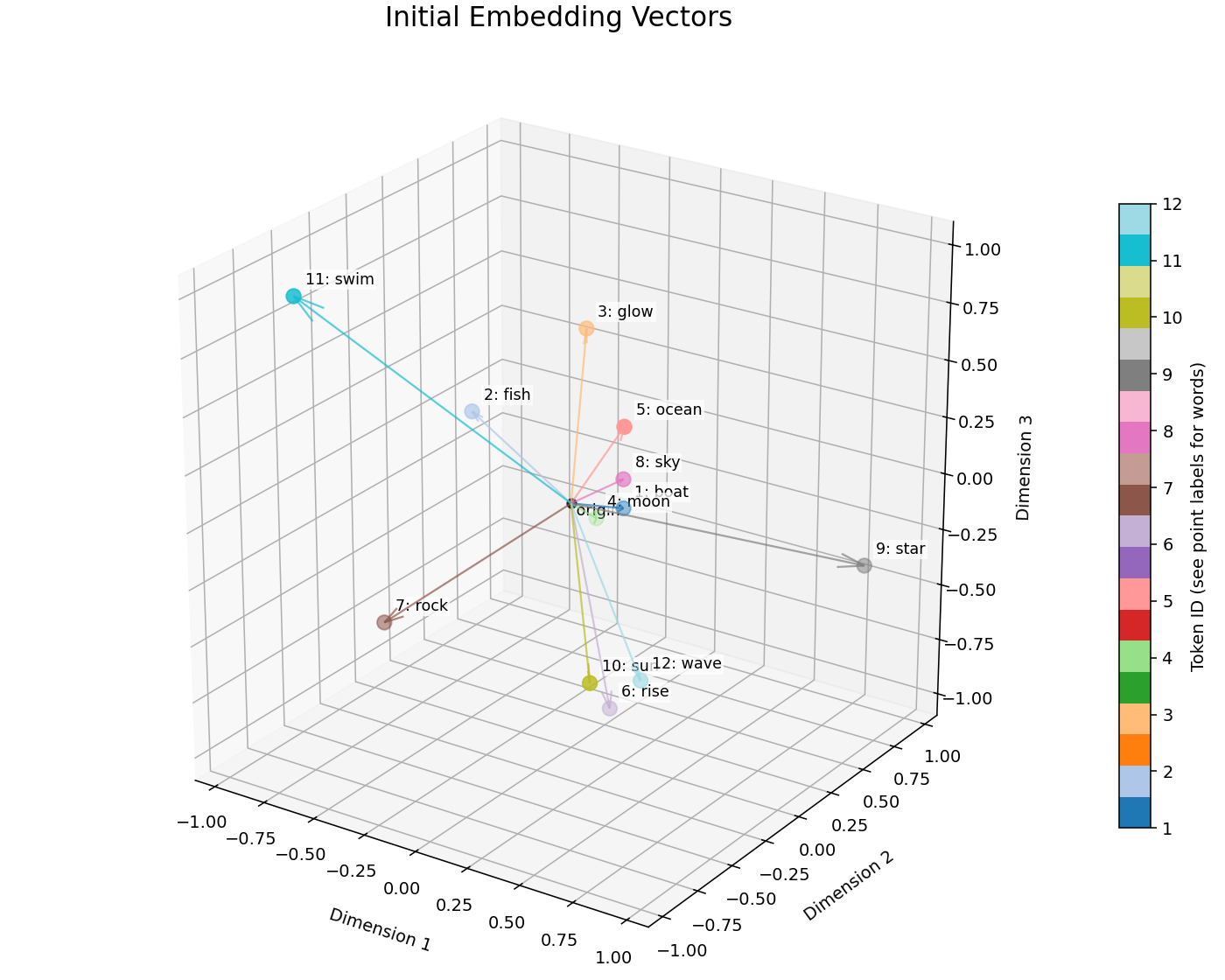
We have our data ready for training, the next step is designing how the training should be done. Since we have converted all input into number, the training steps will involve quite a bit of mathematics.

2. Predict how related two words are
When training the model, the goal is to make the model be able to tell what is right and wrong by itself without any human intervention. We want the model to be able to guess whether a pair of word is related or not. However, since we have converted all input into a vector, how can the model guess if two words are related or not?
With vector, determining its “similarity” is by finding how aligned two vectors are. The alignment can be measured through length and direction of the vector. Take a look at image below.
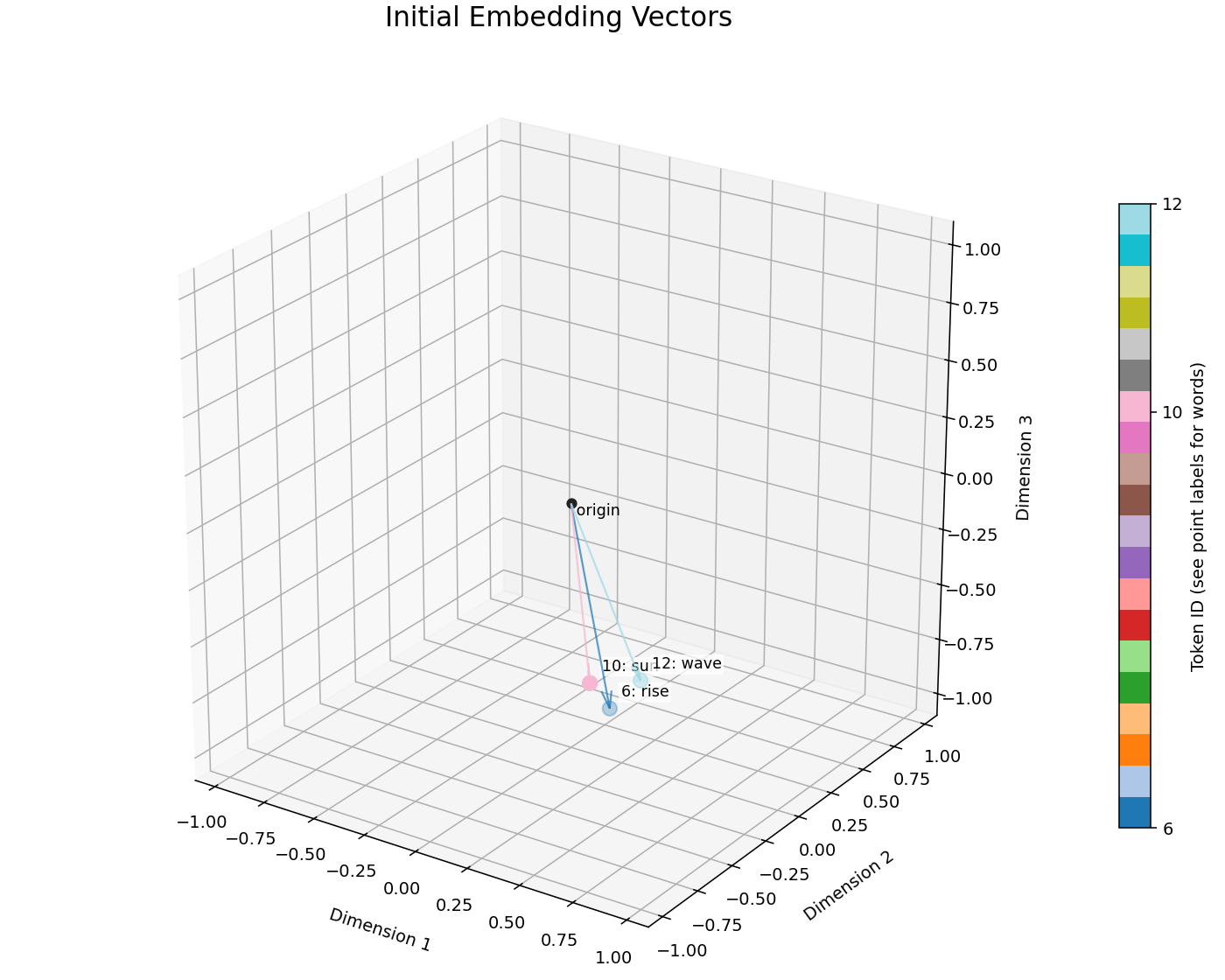
The vectors have different lengths and point in different directions. We can measure the direction of a vector from its angle, the value of θ. So how do we tell if two vectors are aligned or not? We need to measure its alignment and produce a number that the model uses to make its prediction. The vector alignment can be calculated using a formula called dot product:
a ⋅ b = ∑(ai x bi)
So how do we do it? We create a pair of vector, vector A and vector B then we apply it into the formula. Remember that the words now represented as vector, so we pick two words from our dataset.
For every pair of words in the dataset, the model calculates a dot product to produce its current prediction of how related the pair is. The result is the current model prediction on how related these two words are. It reflects the model’s current belief, not what the training data says is correct.
Let’s try one example, we take one line from the dataset, "sun rise glow". After that, from one line, we create a pair of word
starting from ["sun"; "rise"]. The tokenizer would turn this word into a token ID, 10 and 6 respectively, then
we get the vector from these words.
| Token ID | Dimension 1 | Dimension 2 | Dimension 3 |
|---|---|---|---|
| 6 | 0.150 | 0.061 | -0.905 |
| 10 | 0.563 | -0.704 | -0.366 |
Then we apply into dot product formula:
vector A(Rise) ⋅ vector B(Sun) = (0.150 * 0.563) + (0.061 * -0.704) + (-0.905 * -0.366)
vector A(Rise) ⋅ vector B(Sun) = 0.372736
Now that we have the result for dot product of “Sun” and “Rise”. Let’s do a little experiment, what if we pair “Sun” with “Wave” despite it’s not in the same line in the dataset. Token ID for “Wave” is 12, so:
| Token ID | Dimension 1 | Dimension 2 | Dimension 3 |
|---|---|---|---|
| 12 | 0.369 | -0.045 | -0.675 |
| 10 | 0.563 | -0.704 | -0.366 |
Then we apply into dot product formula:
vector A(Wave) ⋅ vector B(Sun) = (0.369 * 0.563) + (-0.045 * -0.704) + (-0.675 * -0.366)
vector A(Wave) ⋅ vector B(Sun) = 0.486477
The result is larger than before. What does that mean? In the dot product, a larger result generally means the two vectors are pointing in a more similar direction. The result is also influenced by the lengths of the vectors, so both the direction and the lengths contribute to the final value. Looking back at Figure 2, we can see that “Sun” forms a smaller angle with “Wave” than with “Rise”. Since the angle is smaller, the dot product between “Sun” and “Wave” becomes larger.
The next question is, is it right? Is word “Sun” related to “Wave”? No, based on the dataset. Yet the number tells vector “Sun” is more aligned with “Wave”. So how can we tell the model this is wrong?
3. Measure how wrong the prediction is
When encountering a wrong prediction, the model is not aware of right and wrong. It’s just doing math formula to calculate how aligned vector A and vector B. Since initially we set the vector as random, the model prediction is only as good as the current value in embedding vector table. So we need to give the model a way to ask “how wrong am I?” and answer it by itself.
The simplest way is to compare the model’s prediction with the correct answer from the dataset.
Calculate Error
How can the model measure how wrong its prediction? We need two things:
- What the model predicts,
- What the dataset says is correct.
The model already has a prediction from the dot product. However, there is one problem. Recall the result from dot product of “Sun” and “Rise” was 0.372736 while dot product of “Sun” and “Wave” is 0.486477. A larger dot product indicates that the model predicts the two words more related. At first glance, we might think we can directly interpret the dot product. For example, we might decide that values greater than X mean the pair is related, while smaller values mean it is unrelated.
The problem is that training does not stop after one update. As the embedding vectors continue to change over many epochs, the dot product can keep increasing. A score that was once 0.48 might later become 10, 20, or even 100. Since there is no fixed upper bound, a value of X that seems reasonable early in training may no longer make sense later.
Instead of comparing these unbounded scores directly, we first convert them into values within a fixed range. One way to do is using a Sigmoid function.
σ(x) = 1 / (1 + e−x)
where e is approximately 2.718
Convert Prediction Value
To put it simply, Sigmoid function will convert the dot product result into a value between 0.0 to 1.0. This converts the dot product into a value that is much easier to interpret and compare with the correct target from the dataset. In this case, a value close to 1.0 means the model predicts the pair is similar, 0.5 means the model is uncertain, and a value close to 0.0 means the pair is unrelated.
Let’s apply Sigmoid function to dot product of “Sun” and “Rise”,
σ(x) = 1 / (1 + 2.718<sup>−0.372736</sup>)
σ(x) = 0.592111
then apply Sigmoid function to dot product of “Sun” and “Wave”,
σ(x) = 1 / (1 + 2.718<sup>−0.486477</sup>)
σ(x) = 0.619264
Now that we have converted the dot product into a value between 0.0 and 1.0, we will use that value as the model’s prediction. We can compare it directly with the target from the dataset.
Now we can use a simple formula to measure how wrong the model prediction is:
error = target - prediction
- error, how wrong the model prediction is
- target, the correct value from the dataset (1.0 for related, 0.0 for unrelated)
- prediction, the model’s predicted value after applying the sigmoid function
Once the model knows it’s wrong, how does it become less wrong?
4. Update the vectors
After the model measures how wrong its prediction after making a prediction, the model needs to know how to reduce the error. The only way to reduce it is by changing the prediction score to be closer to target.
We don’t need to change the target, nor the dataset, only the vectors since we calculate the prediction using dot product. Therefore, we will use the error to update the vectors.
Recall that the dot product is influenced by both the direction and the lengths of the two vectors. Hence, changing a vector changes the dot product. This can be done by updating vector A in the direction of vector B. As a result, the direction of vector A gradually becomes more aligned with vector B, while its length may also change during training.
We can update the vector using the following formula:
Vector A(i) = Vector A(i) + error × Vector B(i)
This formula can be read as: “Take Vector A and add a portion of Vector B.” The error determines how much of Vector B is added. If the error is positive, Vector A is updated toward the direction of Vector B. If the error is negative, it is updated in the opposite direction, making the vectors less aligned. As the vectors become more aligned, their dot product increases.
Let’s try updating the pair of “Sun” and “Rise” here,
| Dimension | Vector A (Sun) | Error | Vector B (Rise) | New Vector A |
|---|---|---|---|---|
| 1 | 0.563 | 0.407889 | 0.150 | 0.624183 |
| 2 | -0.704 | 0.407889 | 0.061 | -0.679119 |
| 3 | -0.366 | 0.407889 | -0.905 | -0.73514 |
Once we updated vector A, let’s use the new Vector A to calculate using dot product to see if there is any improvement
Vector A(Sun) ⋅ Vector B(Rise) = (0.624183 * 0.150) + (-0.679119 * 0.061) + (-0.73514 * -0.905)
Vector A(Sun) ⋅ Vector B(Rise) = 0.717503
Sigmoid(0.717503) = 0.672041
Well, that’s an improvement. Previously we got 0.592111 and now we get 0.672041. This shows the model gains more confidence in its prediction. What about the wrong pair of “Sun” and “Wave” ? We follow the same steps but the only different is we set the target to 0.0 because we want the similarity to be as low as possible.
Preventing Large Updates
Now the model knows how to reduce the error, yet there is one other problem we still need to fix. Every prediction is immediately followed by an update to a vector during training. If we have eight lines of text in the dataset, training starts from the first line and updates the vectors sequentially. The word “Sun” in the dataset is placed on the same line with words “Rise”, “Glow”, and “Ocean”. We have the following in the dataset:
- Line 1, “sun rise glow”
- Line 7, “sun glow ocean”
After updating “Sun” to become more aligned with “Rise”, the next training pair may update it again to become more aligned with “Glow”, then with “Ocean”. Each update helps the current pair but can partially undo a previous one.
This will cause a problem on the next training step, it may move the vector too far again to another direction. Instead of making small adjustments, the vector keeps making large jumps. So how do we prevent this? We simply tell the model to make a smaller update. How? By adding another small number in the formula we use to update the vector. This number is called Learning Rate.
While there are many techniques to specify learning rate, we focus on main purpose here: to make each update smaller so the vector changes more carefully during training. Hence, the formula is:
Vector A(i) = Vector A(i) + learning rate * error × Vector B(i)
The value of Learning Rate here can be anything, as long as it doesn’t cause the problem we have discussed. I used 0.1 as a start and then adjust the epochs to get a better result of the training.
Training Results
After many epochs, related word vectors gradually become more aligned, allowing the model to predict relationships between words more accurately based on the training dataset. This is how embedding vectors for “Sun”, “Rise”, and “Wave” look like now after training:
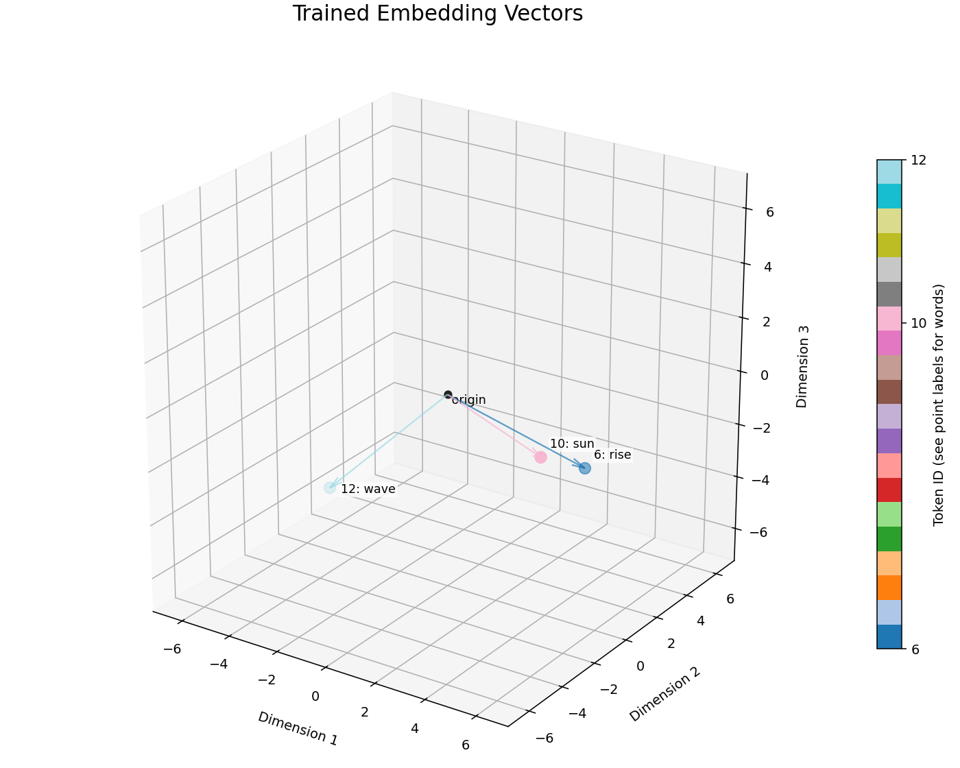
When comparing with Figure 2, we notice that “Sun” is now more aligned with “Rise” than with “Wave”. This shows the model is able to predict the relationships between words better. Figure 3 only shows one example involving “Sun”. If we look at all of the word vectors after training, we can see the same pattern across the entire vocabulary in the following figure.
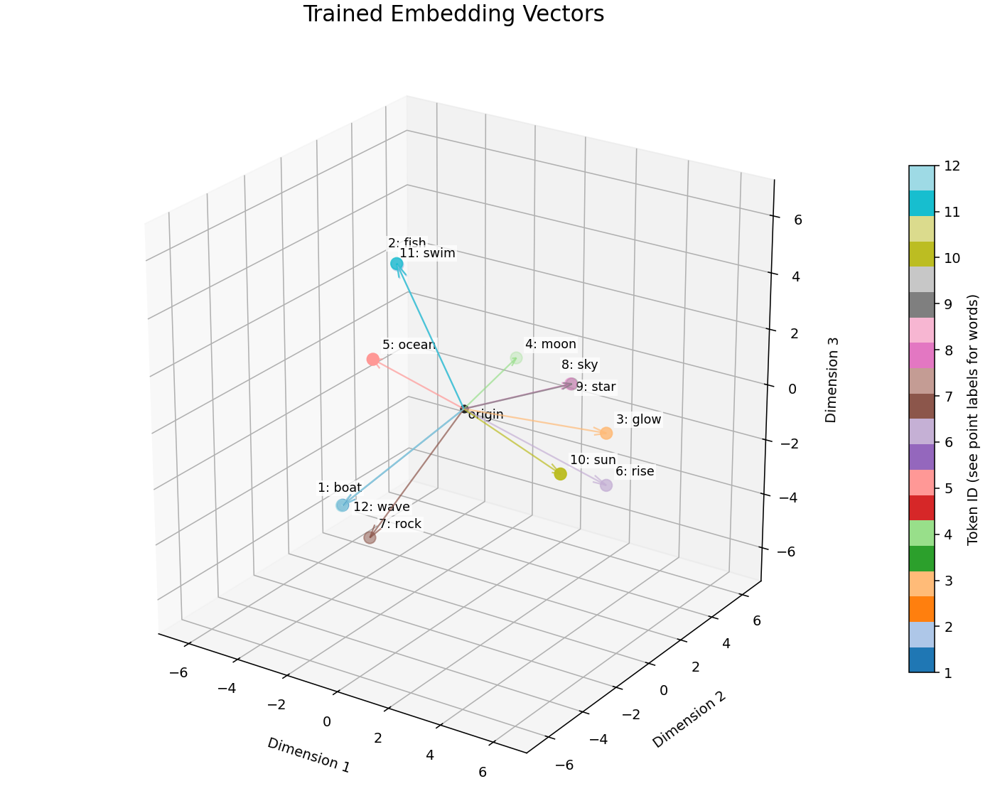
Notice that “Sun”, “Rise”, and “Glow” now point in similar directions. “Ocean” also points in a roughly similar direction, although not as closely aligned. This is expected because the word “Ocean” appears with “Sun” in one sentence, but it also appears with words such as “Fish”, “Swim”, “Wave”, and “Boat”. The final position of each vector reflects all of the relationships the model learned during training, not just a single word pair.
Now the vectors are no longer mysterious. They start as random numbers, and repeated prediction, error measurement, and small corrections gradually organize them into meaningful positions.
Since the vectors have meaningful positions, how does the model measure the similarity between two vectors?
Calculating Similarity
During training, we used the dot product to predict how related two words were. After each prediction, we updated one vector by adding a portion of another, which changed both its direction and its length. The goal, however, is to make vectors of related words point in similar directions. The change in vector length is simply a side effect of the update process. As shown in Figure 4, the vectors do not necessarily have the same length, yet they point in similar directions.
Can we compare only the direction of two vectors? Yes. Instead of comparing both length and direction, we use a formula called Cosine Similarity, which measures how closely two vectors point in the same direction while ignoring their lengths.
Cosine similarity ranges from -1.0 to 1.0. A value close to 1.0 means two vectors point in nearly the same direction, a value close to 0 means their directions are unrelated, and a value close to -1.0 means they point in opposite directions.
To see how this works, let’s compare the word “Sun” with the other words in the trained embedding.
| Word | Cosine Similarity |
|---|---|
| Glow | 0.905 |
| Rise | 0.811 |
| Ocean | 0.426 |
| Fish | -0.188 |
| Swim | -0.190 |
The result matches what we observed in Figure 4. The vectors of “Glow” and “Rise” point in nearly the same direction as “Sun”, so they receive high similarity scores. Although “Rise” has a different vector length from “Sun”, it is still considered similar because cosine similarity compares only their directions.
The word “Ocean” still has a positive similarity because it appears together with “Sun” in the dataset. However, its score is lower because “Ocean” also appears with words such as “Fish”, “Swim”, “Wave”, and “Boat”. These additional relationships pull its vector toward a different direction, making it less aligned with “Sun” than “Glow” or “Rise”.
Finally, “Fish” and “Swim” receive negative similarity scores because their vectors point in almost the opposite direction from “Sun”. Even though they are related to “Ocean”, they do not appear in similar contexts as “Sun”, so the model places them in a different region of the embedding space.
Final Answers
We’ve now seen how embedding vectors are created and how the model uses them to measure similarity. Let’s revisit the questions we started with.
- How are those numbers produced?
They are not assigned manually. Each word starts with a random vector. During training, the model repeatedly predicts relationships between words, measures its error, and updates the vectors. After many iterations, the vectors gradually move into positions that reflect the relationships learned from the training data.
- What do they mean to the model?
The model does not understand words the way humans do. Instead, it represents each word as a vector. Individually, the numbers are meaningless. Together, however, they determine a word’s position in the embedding space. The model compares these positions mathematically to estimate how closely different words are related.
- If those numbers are just random, why don’t we just assign a random number for each word instead of using an embedding model?
Random vectors contain no useful information. Training gradually adjusts them so that words appearing in similar contexts move closer together. The final vectors therefore represent patterns the model learned from the dataset rather than arbitrary numbers.
I have written the simple POC program here. Understanding these ideas takes time. By the time I finished writing this article, newer models had already been released. I haven’t touched the transformer yet to understand when the model stops paying attention, and also how tool calling works. I hope this also gives a broader perspective on how vectors play such an important role in language models. Let’s keep learning the principles first!